Studies can be designed to be robust to missing data, such that any missingness will have a limited effect and bias on any results. Frequently, this is not possible. Thus, this sub-chapter provides an overview of some missing data handling methods. Additionally, discussing these methods can quickly get very technical; we will do our best to avoid using jargon and leave the technical explanations to the great, already existing, resources out there, linked in Checklist and Resources.
Deletion
The simplest way of handling missing data would be to remove any rows or data entries that have missing values in any variables of interest. This is also known as listwise deletion and complete-case analysis Oluwaseye Joel et al., 2022. However, this may greatly reduce the available data for analyses, introduce or increase bias, and decrease representation Woods et al., 2024. Nevertheless this is an appropriate option MCAR data.
Pairwise deletion, or available case analysis, only involves removing data entries as the need arises Pigott, 2001. This method does allow using more of your data, but has a lack of consistency in results and can result in one or more variable being explained by others (via a linear combination).
Imputation
Imputation refers to “filling in” any missing values. Many ways of imputing missing data exist:
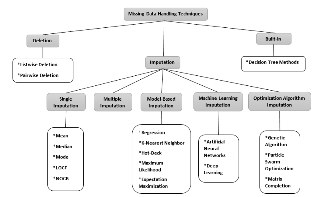
Figure 1:Diagram of missing data handling techniques, created by Joel et al. Oluwaseye Joel et al., 2022. Abbreviations: LOCF - Last Observation Carried Forward, NOCB - Next Observation Carried Backward.Used under a CC-BY 4.0 licence. DOI: 10.15157/IJITIS.2022.5.3.971-1005.
Single imputation involves imputing a single value per missing value. These methods are easy to implement and suitable when there are a small number of missing values in a large dataset.
In contrast, multiple imputation methods can generate several values for each missing value. This means that multiple imputation methods can also have an average value and variance assigned to each imputed value, thereby giving the option to test the stability of downstream analyses. One popular multiple imputation method is Multivariate Imputation by Chained Equations (MICE), which is explained below.
The more complicated imputation methods, such as those under the model-based, machine learning and optimization algorithm imputation headings tend to perform better when there are many missing values and can handle many types of missing data. These are harder to implement and usually require very large sample sizes to produce consistent results.
Great care should be taken with imputation methods, as they may introduce or further amplify existing bias. For instance, in our sample dataset, those with the most severe cognitive decline were unable to attend the follow-up visit to get their cognition assessed. If their values were imputed using everyone else’s, their values would be considerably lower than in reality.
MICE
MICE works iteratively to impute data. It uses the most complete data to inform the values of increasingly less complete entries. This is done iteratively in cycles, such that at the end of each cycle there is one set of imputed values Buuren & Groothuis-Oudshoorn, 2011. A slightly more detailed explanation follows below.
The first step of a cycle involves filling in the missing values of all variables, using a simple method. Then, the variable with the least number of missing values are set back to missing. The observed values of that variable are regressed on variables in the rest of the dataset. Imputed values are then estimated using this regression model, and the missing values are replaced Azur et al., 2011. A different type of regression can be used for each variable, such that each variable is handled separately and can be assigned a unique distribution. This imputation also includes some randomness to capture the uncertainty of the imputed Wulff & Jeppesen, 2017. Next, the variable with the 2nd least number of missing values are set back to missing and imputed as described previously, and so on. This is done iteratively, even after all missing values have been imputed. At the end of a set number of iterations over all variables (for example, 50 iterations), the cycle is complete and each missing value now has an unbiased estimated imputed value.
Often, MICE is done repeatedly, such that an average value and variance are obtained per imputed value. Therefore, 5 cycles may be completed, so that there are 5 imputed values per missing data point. Simulations can also be used to estimate the performance of MICE in a given dataset, and determine whether values are imputed within a certain tolerance. Another method of evaluating the imputation is by comparing the distributions of the original and the imputed data. If the distributions are quite similar, then the imputed values match.
Example Imputation
Below we provide code implementation of imputing missing values in our example dataset (introduced in Missing Data Structures) using the R mice package Buuren & Groothuis-Oudshoorn, 2011:
# use mice to create 5 imputed datasets (m=5) using predictive mean matching (meth='pmm') and 50 maximum iterations
temporary_dataset <- mice(fictional_dataset,m=5,maxit=50,meth='pmm',seed=500)
# impute the values using the first of the five datasets
imputed_dataset <- complete(temporary_dataset,1)
Which has the following output:
| Participant Number | Age | Diastolic Blood Pressure | Systolic Blood Pressure | Blood Test Result | Motor Score | Cognitive Score |
|---|---|---|---|---|---|---|
| 1 | 56 | 82 | 118 | Positive | 10 | 35 |
| 2 | 78 | 87 | 134 | Negative | 32 | 29 |
| 3 | 85 | 83 | 134 | Negative | 27 | 22 |
| 4 | 43 | 83 | 121 | Negative | 15 | 36 |
| 5 | 67 | 86 | 131 | Positive | 20 | 25 |
| 6 | 82 | 92 | 133 | Negative | 26 | 22 |
| 7 | 88 | 92 | 133 | Positive | 34 | 25 |
| 8 | 71 | 87 | 133 | Negative | 33 | 22 |
The average of all 5 imputed datasets is as follows:
| Participant.Number | Age | Diastolic Blood Pressure | Systolic Blood Pressure | Blood Test Result | Motor Score | Cognitive Score |
|---|---|---|---|---|---|---|
| 1 | 56 | 82 | 118 | Negative | 10 | 35 |
| 2 | 78 | 87 | 134 | Negative | 32 | 29 |
| 3 | 85 | 83 | 131 | Negative | 27 | 28 |
| 4 | 43 | 83 | 121 | Positive | 15 | 36 |
| 5 | 67 | 86 | 131 | Positive | 20 | 25 |
| 6 | 82 | 92 | 133 | Positive | 26 | 28 |
| 7 | 88 | 87 | 127 | Positive | 34 | 29 |
| 8 | 71 | 86 | 133 | Positive | 33 | 22 |
where for the blood test results, the most common value was chosen. The variance of the missing values was:
| Participant Number | Diastolic Blood Pressure | Systolic Blood Pressure | Cognitive Score |
|---|---|---|---|
| 3 | 1.52 | 5.50 | 7.22 |
| 6 | 0.00 | 0.00 | 6.69 |
| 7 | 3.58 | 7.16 | 6.11 |
| 8 | 1.79 | 1.22 | 0.00 |
Therefore, the variance was quite high. However, this is not the ideal dataset to be using MICE. In fact, MICE is suited best for MAR data and as we know our example dataset has all 3 types of data missingness.
In a more realistic dataset, the function parameters can be adjusted to improve the estimated values. For instance, the method of imputation can be changed to a Bayesian linear regression of multilevel model if this would be more appropriate for your data. It may also be more appropriate to create more imputed datasets, if there is a high level of missingness in the data White et al., 2011. MICE has been thoroughly developed and implemented in R. It is even easy to pool the results of downstream analyses, by fitting a model to each of the imputed datasets and then combining the results together.
Using MICE in python is also available, but is an experimental feature available in scikit-learn, via the IterativeImputer class:
# explicitly require this experimental feature to use IterativeImputer
from sklearn.experimental import enable_iterative_imputer
# now you can import normally from sklearn.impute
from sklearn.impute import IterativeImputer

# Remap "Blood Test Result" column, so it is expressed as a number and is compatible with IterativeImputer
df_fictional_dataset['Blood Test Result'] = df_fictional_dataset['Blood Test Result'].replace({'Negative': 0, > 'Positive': 1})

# initialize the imputer
imp = IterativeImputer(max_iter=50, random_state=500, sample_posterior=True, keep_empty_features=False)
# train and fit the imputer in one step
imputed_values = imp.fit_transform(df_fictional_dataset)

# instantiate dataframe by copying original
df_imputed_dataset = df_fictional_dataset.copy()
# replace values in dataframe based on fit_transform output
df_imputed_dataset.iloc[:, :] = imputed_values
which gives us:
| Participant Number | Age | Diastolic Blood Pressure | Systolic Blood Pressure | Blood Test Result | Motor Score | Cognitive Score |
|---|---|---|---|---|---|---|
| 1 | 56 | 82 | 118 | Positive | 10 | 35 |
| 2 | 78 | 87 | 134 | Positive | 32 | 29 |
| 3 | 85 | 85 | 155 | Positive | 27 | 23 |
| 4 | 43 | 83 | 121 | 0 | 15 | 36 |
| 5 | 67 | 86 | 131 | 1 | 20 | 25 |
| 6 | 82 | 92 | 133 | 0 | 26 | 91 |
| 7 | 88 | 107 | 157 | 1 | 34 | 30 |
| 8 | 71 | 64 | 127 | 0 | 33 | 22 |
The IterativeImputer class allows for both univariate and multivariate imputations and encompasses many different imputation methods (function parameters specify which is being used). The training step of the imputer can also be done separately to fitting (by using the imp.fit function first, and then imp.transform). This means that the training dataset can also be different to what is then provided to be imputed.
In the example above, we are showing the results from one MICE cycle. In order to obtain several cycle results (or multiple imputed values), then you need to manually apply it several times with different random seeds when sample_posterior=True. This is not shown here for brevity.
Summary
Indeed, this is a very vast area of research, with many proposed methods available; if you are interested in finding out more please see Checklist and Resources. Hopefully, this sub-chapter acts as a useful starting point!
- Oluwaseye Joel, L., Doorsamy, W., & Sena Paul, B. (2022). A Review of Missing Data Handling Techniques for Machine Learning. International Journal of Innovative Technology and Interdisciplinary Sciences, 5(3), 971–1005. 10.15157/IJITIS.2022.5.3.971-1005
- Woods, A. D., Gerasimova, D., Van Dusen, B., Nissen, J., Bainter, S., Uzdavines, A., Davis-Kean, P. E., Halvorson, M., King, K. M., Logan, J. A. R., Xu, M., Vasilev, M. R., Clay, J. M., Moreau, D., Joyal-Desmarais, K., Cruz, R. A., Brown, D. M. Y., Schmidt, K., & Elsherif, M. M. (2024). Best practices for addressing missing data through multiple imputation. Infant and Child Development, 33(1), e2407. https://doi.org/10.1002/icd.2407
- Pigott, T. D. (2001). A Review of Methods for Missing Data. Educational Research and Evaluation, 7(4), 353–383. 10.1076/edre.7.4.353.8937
- van Buuren, S., & Groothuis-Oudshoorn, K. (2011). mice: Multivariate Imputation by Chained Equations in R. Journal of Statistical Software, 45(3), 1–67. 10.18637/jss.v045.i03
- Azur, M. J., Stuart, E. A., Frangakis, C., & Leaf, P. J. (2011). Multiple imputation by chained equations: what is it and how does it work? [Journal Article]. Int J Methods Psychiatr Res, 20(1), 40–49. 10.1002/mpr.329
- Wulff, J. N., & Jeppesen, L. E. (2017). Multiple imputation by chained equations in praxis: Guidelines and review. Electronic Journal of Business Research Methods, 15(1), 41–56.
- White, I. R., Royston, P., & Wood, A. M. (2011). Multiple imputation using chained equations: Issues and guidance for practice [Journal Article]. Stat Med, 30(4), 377–399. 10.1002/sim.4067